Distributed Reinforcement Learning: A draft
These last few months, I have been working on deep reinforcement learning (RL), a very active research area of artificial intelligence. Although RL algorithms are not so easy to understand, I was amazed by the simplicity of the RL control loop:


If you have never listened to RL, I will explain quickly: every RL problem can be expressed as a system consisting of an agent and an environment. The environment produces an initial state, which describes the initial configuration of the system. Then, our agent interacts with an environment by observing the state, and using this information, the agent selects an action. Finally, the environment receives the action and transitions into the next state, returning the next state and a reward to the agent. We repeat this process until we reach an objective, that it is commonly defined as the sum of rewards received by the agent.
However, this RL control loop has some drawbacks, and the main which I consider more important is the exploration-exploitation dilemma, that is to say, we need to find a balance between explore new options (which can seem not so optimal at the beginning) or exploit the best option based on our current knowledge (which can be suboptimal due to incomplete information).
And at this point, I had a question:
Can we decrease the impact of exploration-exploitation dilemma if we train several independent agents?
Obviously, this problem has several (and good) partial solutions, like epsilon-greedy exploration [1] or Thomson sampling [2]. However, I consider that this is a good opportunity to test how distributed deep learning can be used beyond a tool to train quickly with less high-performance hardware, so we don’t lose anything by trying; after all, this is a draft.
Policy-gradient methods: a short introduction
In the introduction, we defined the concept of action as the response of the agent to the environment. We will call the function that takes the environment’s states and produces agents’ actions a policy, which we commonly denote as $ \pi $.
Formally, we can define the terms of state, action and reward as follows:
\[\begin{align} &s_t \in \mathcal{S} \text{ is the state, } \mathcal{S} \text{ is the state space.} \\ &a_t \in \mathcal{A} \text{ is the action, } \mathcal{A} \text{ is the action space.} \\ &r_t = \mathcal{R}(s_t, a_t, s_{t+1}) \text{ is the reward, } \mathcal{R} \text{ is the reward function.} \end{align}\]The tuple $ (s_t, a_t, s_{t+1}) $ is called transition, and is the combination of the previous state, the action that it produced, and the current state (result of $s_t$ and $a_t$). Our objective in RL is to correctly predict the next action given a history of states and actions; it is to say
\[s_{t+1} \sim P(s_{t+1} | (s_0, a_0), \dots, (s_t, a_t)).\]Nevertheless, in practice, we use the Markov property, and with this assumption, our problem simplifies to
\[s_{t+1} \sim P(s_{t+1} | s_t, a_t).\]And our objective is to maximize the return $ R(\tau) $ of our trajectory $ \tau = (s_0, a_0, r_0), \dots, (s_T, a_T, r_T) $:
\[R(\tau) = r_0 + \gamma r_1 + \gamma^2 r_2 + \cdots + \gamma^T r_T = \sum_{t=0}^T \gamma^t r_t.\]As we can see, this is a discounted sum of the rewards in a trajectory of decisions, where $ \gamma \in [0, 1] $ is a hyperparameter which controls the discount factor.
At this point, we have several paths we can follow:
- Find a policy that maps states to actions: $ a \sim \pi(s) $.
- Find a value function $ V^\pi(s) $ or $ Q^\pi(s, a) $ to estimate the expected return $ R(\tau) $.
- Find an environment model $ P(s’ | s, a) $.
In this case, we will proceed with the first option that may not be the most optimal (models like deep Q-learning [3] have demonstrated a good performance on several tasks). This kind of models is often called policy-based methods.
The advantage of these kinds of methods is that, in general, they are quite intuitive: if our agent needs to act in an environment, it makes sense to learn a good policy. And if you remember the Markov property, the next state in a determinate state depends on the current state and the action that we take at this moment, so our action must be determinate only by the current state, that is, $ a \sim \pi(s) $.
REINFORCE
The REINFORCE algorithm [4] is one of the most used algorithms in policy-based methods. As we said above, we need to learn a parametrized policy $ \pi_\theta $ that maximizes the expected return:
\[J(\pi_\theta) = \mathbb{E}_{\tau\sim\pi_\theta}[R(\tau)] = \mathbb{E}_{\tau\sim\pi_\theta} \left[\sum^T_{t=0} \gamma^tr_t\right]\]Actually, the policy $ \pi_\theta $ gives us a distribution, and from this distribution we are going to sample the next action to take (exploration). But if we note that one action is beneficial, we try to increase this action (exploitation).
To maximize the probability of the best actions, we use gradient ascent:
\[\theta \leftarrow \theta + \alpha\nabla_\theta J(\pi_\theta).\]Where the term $ \nabla_\theta J(\pi_\theta) $ is known as the policy gradient. However, in practice, libraries like PyTorch works better in minimization problems, and for this reason we instead use a surrogate objective, namely $ -\log \pi_\theta(a | \theta) $, which has a larger range, and instead of maximizing it, the objective is minimizing it.
Unfortunately, deriving the equation of gradient descent for REINFORCE deserves its own post, and fortunately, there are a lot of resources on the internet about this topic. I highly recommend you read the Lil’Log post. I’ll hope in the future to publish my own compendium on Reinforcement Learning from a theoretical point of view in the future, but for the moment, let’s focus on the distributed model.
One policy to rule them all: the parameter server model


Before jumping to the implementation, we need to plan what we expect from our model. Although the objective is to train several agents, all of them will share the same policy. Every agent will pull the policy from our primary server, and with this policy will elapse a period in its own (independent) environment to obtain the gradients to optimize the policy. However, the model will not update the policy’s weights; instead, it’s going to push the gradients to the central server that will be in charge of updating the model.
Remember that you can find the complete version of my implementation on my GitHub repository. This is only the first part of this project, so stay tuned for new and better updates.
For this purpose, we are going to use a simplified version of the parameter server model [5]. The Parameter Server (PS) architecture is a widely used model for distributed machine learning, where the model parameters (weights and biases) are stored on a central server, and the computation and data are distributed across multiple worker nodes.


As you can see in the image above, PS hast two types of computers: the server and the workers. The server only holds the current model parameters, while the workers are responsible for processing data and computing the gradients that are sent to the server.
In PS, we can work with synchronous or asynchronous updates; however, asynchronous updates require more metadata to carry on backpropagation since we can have staleness problems. In the synchronous setting, all the workers wait for all gradients to be aggregated before updating the parameters; that is to say, every worker will use the same set of parameters.
The server
Let’s start with the server, whose only job is to maintain and update the parameters of our policy. In this work, I use PyTorch Distributed. In PyTorch Distributed, every node must be aware of two things: What is the world size? (i.e., how many nodes do we have), and what is its rank?
By convention, the node with rank 0 is always the coordinator, that is, the parameter server, and this coordinator will receive the policy and other hyperparameters useful for training. However, it is important to separate the gradients (__gradients variable) for the model. Also, we are going to need a “space” to receive the gradients of every worker (____gradients_buffer variable).
1
2
3
4
5
6
7
8
9
10
11
12
13
14
15
class ParameterServer:
    def __init__(self, world_size: int, policy: nn.Module, lr: float = 0.001, max_episodes: Optional[int] = None):
        self.policy = policy.to(torch.device("cpu"))
        self.running_reward = 0
        self.__optimizer = torch.optim.Adam(self.policy.parameters(), lr=lr)
        self.__max_episodes = max_episodes

        self.__gradients = []
        self.__worker_buffer = []
        for param in self.policy.parameters():
            worker_return = []
            for _ in range(world_size):
                worker_return.append(torch.empty(param.size()))
            self.__worker_buffer.append(worker_return)
            self.__gradients.append(torch.empty(param.size()))
Next, we need a method to broadcast our parameters. In this case, it is simple: the communication API gives us a method to broadcast tensors easily, so it is not difficult to do that:
1
2
3
4
5
class ParameterServer:
    ...
    def _broadcast_parameters(self):
        for param in self.policy.parameters():
            dist.broadcast(param.detach(), src=0)
The next step is a little bit complicated, we need to gather all the worker’s gradients in our server. Again, we have a method which does it, dist.gather receives a list of tensors (one for every node, including the coordinator) and we need to receive this list for every parameter in our model. When we have all our gradients for one parameter, we reduce them (except the first one, that is the dummy gradient of the server) summing all the gradients and saving it in the __gradients variable.
1
2
3
4
5
6
7
class ParameterServer:
    ...
    def _receive_gradients(self):
        for idx, param in enumerate(self.policy.parameters()):
            dummy_grad = torch.empty(param.size())
            dist.gather(dummy_grad, self.__worker_buffer[idx], dst=0)
            self.__gradients[idx] = reduce(lambda x, y: x + y, self.__worker_buffer[idx][1:])
Once we have our gradients, we need to apply this information to our policy. Luckily, all the information that PyTorch needs to backpropagate the gradients is contained in the grad variable of our tensor:
1
2
3
4
5
6
class ParameterServer:
    ...
    def _update(self):
        for idx, param in enumerate(self.policy.parameters()):
            param.grad = self.__gradients[idx]
        self.__optimizer.step()
And that’s all for our server; we only need to repeat the process bradcast -> receive -> update for every episode in our training process.
1
2
3
4
5
6
7
8
9
class ParameterServer:
    ...
    def run(self):
        iterator = range(self.__max_episodes) if self.__max_episodes is not None else count(1)
        for _ in tqdm(iterator):
            self.policy.train()
            self._broadcast_parameters()
            self._receive_gradients()
            self._update()
The workers
The workers have more logic behind their operation. For the distributed agent (which will be our worker), we need to specify the discount factor $ \gamma $, the policy, the environment (in this case, I am using Gymnasium) and a buffer for our parameters (__parameter_buffer variable). This parameter buffer will be filled with a skeleton of every parameter.
1
2
3
4
5
6
7
8
9
10
11
12
13
14
15
16
17
18
19
class DistAgent(Agent):
    def __init__(self, policy: nn.Module, env: str, max_iters: int, gamma: float,
                 device: torch.device = torch.device("cpu")):
        super().__init__(policy, device)
        self._device = device
        self._max_iters = max_iters
        self._gamma = gamma

        self.policy = policy.to(self._device)
        self.env = gym.make(env)
        self.running_reward = 0

        self.__parameter_buffer = {}
        self.__rewards = []
        self.__actions = []

        for name, param in self.policy.named_parameters():
            if param.requires_grad:
                self.__parameter_buffer[name] = torch.empty(param.size(), dtype=param.dtype)
Before we start a new episode, we need to fetch the new policy’s parameters. We use the same dist.broadcast method, that when we call it in a node with a different rank of the source, it receives instead of sending the tensors. And when we receive all the parameters, we update the state dict of the policy with this new data.
1
2
3
4
5
6
7
8
9
10
11
class DistAgent(Agent):
    ...
    def fetch(self):
        for param in self.__parameter_buffer:
            dist.broadcast(self.__parameter_buffer[param], src=0)

    def update(self):
        self.fetch()
        for name in self.__parameter_buffer:
            self.__parameter_buffer[name].to(self._device)
        self.policy.load_state_dict(OrderedDict(self.__parameter_buffer))
Now it is time to create a method to run an episode. Before we start with a new episode, we need to call update to get the last values for our policy; when we have our policy updated, we start the RL control loop:
- First, we reset our environment.
- For every iteration, we select an action. This action is the result of our sampling process, and with this action, we update our environment and save our reward. This process is repeated until we reach the maximum number of iterations, or we failed in our task.
- We then compute our running reward (how well we have done it in history) and our returns, which we use to compute our loss.
- With our loss, we call the method
backwardto compute the gradients for only this agent and report them to our server.
1
2
3
4
5
6
7
8
9
10
11
12
13
14
15
16
17
18
19
20
21
22
23
24
25
26
27
28
29
30
31
32
33
34
35
36
37
38
39
40
class DistAgent(Agent):
    ...
    def select_action(self, state: np.ndarray):
        action, log_prob = self.act(state)
        self.__actions.append(log_prob)
        return action

    def run_episode(self):
        self.update()

        state, _ = self.env.reset()
        for _ in range(self._max_iters):
            action = self.select_action(state)
            state, reward, done, _, _ = self.env.step(action)
            self.__rewards.append(reward)
            if done:
                break

        reward = sum(self.__rewards)
        self.running_reward = 0.05 * reward + (1 - 0.05) * self.running_reward

        R = 0
        returns = []
        for r in self.__rewards[::-1]:
            R = r + self._gamma * R
            returns.insert(0, R)
        returns = torch.Tensor(returns)
        returns = (returns - returns.mean()) / (returns.std() + 0.001)

        loss = []
        for log_prob, R in zip(self.__actions, returns):
            loss.append(-log_prob * R)
        loss = torch.stack(loss).sum()
        loss.backward()
        self.send_grads()

        del self.__actions[:]
        del self.__rewards[:]

        return reward
And that’s all. We can proceed with our test to see if our distributed model works :)
Results
It’s time to test our little project! Fortunately, we can do it using only one computer (with enough resources), but if you want, you can test it on the cloud using VM instances like EC2. I coded a script that launches our server and several instances of workers using PyTorch Multiprocessing, you can find it on my GitHub Repo.
For example, if you want to run five workers, you must execute the next command in the directory that contains the project (after installing the dependencies):
1
foo@bar:~$ python scripts/launcher.py --workers 5 --max_episodes 200 --master_port 8989
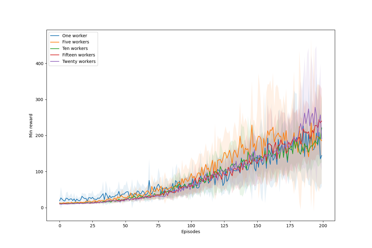
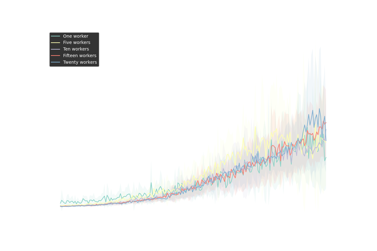
To test our distributed model, we are going to use one, five, ten, and fifteen workers and train them all only during 200 episodes, using the same number of iterations and the same policy network. I present you with a video with my results:
As you can see, with more workers, we obtain better results, as we expected. That is, the exploration is better done using distributed policy with more workers, and the required epochs are less than those required for only one worker. However, a problem with policy-gradient methods is that we have a high variance between models. If you run several times the same script with the same number of workers, it will be times that the performance is worse or better. However, in general, we are going to see that the performance will be better with more workers almost on all occasions, and the time in training is almost always the same because we take advantage of all computer resources.
This is only an introduction to one distributed RL model that maybe is not the best compared to other proposals like GORILA [6], A3C [7] or APE-X [8], but it is a simple one, and I hope I have illustrated how these models can be implemented using only the PyTorch ecosystem. Wait for the next post where I’m going to talk more about these three architectures that I mentioned before; the goal of the year will be to recreate them using the smallest number of dependencies!
References
- [1]M. Wunder, M. L. Littman, and M. Babes, “Classes of multiagent q-learning dynamics with epsilon-greedy exploration,” in Proceedings of the 27th International Conference on Machine Learning (ICML-10), 2010, pp. 1167–1174.
- [2]S. Agrawal and N. Goyal, “Analysis of thompson sampling for the multi-armed bandit problem,” in Conference on learning theory, 2012, pp. 39–1.
- [3]V. Mnih et al., “Human-level control through deep reinforcement learning,” nature, vol. 518, no. 7540, pp. 529–533, 2015.
- [4]R. J. Williams, “Simple statistical gradient-following algorithms for connectionist reinforcement learning,” Machine learning, vol. 8, pp. 229–256, 1992.
- [5]M. Li et al., “Scaling distributed machine learning with the parameter server,” in 11th USENIX Symposium on operating systems design and implementation (OSDI 14), 2014, pp. 583–598.
- [6]A. Nair et al., “Massively parallel methods for deep reinforcement learning,” arXiv preprint arXiv:1507.04296, 2015.
- [7]V. Mnih et al., “Asynchronous methods for deep reinforcement learning,” in International conference on machine learning, 2016, pp. 1928–1937.
- [8]D. Horgan et al., “Distributed prioritized experience replay,” arXiv preprint arXiv:1803.00933, 2018.